
 | So you looked at your test for your Grade 12 Data Management and you have no idea what to do? Check out this mega review list. |
A great emphasis of this course is on Permutations, Combinations and Probability. From unit 3 to unit 5 of the McGraw Hill Ryerson Grade 12 Mathematics of Data Management Book.
A another focus is the knowledge of one variable analysis( such as sampling techniques and types of bias) and two variable analysis (such as finding the correlation coefficient, and cause and effect.)
The last section is about Probability Distributions.
It is usually recommended to start with permutations, combinations and probability and then move on the data types and correlation, last study probability distributions.
Here is a list of key points each units of the course ( Source: onstudynotes.com)
If you found yourself understand each point, you are ready for the test, and able to get 90% + percent. If you feel you could only understand about 70- 80%, you need to crash study for 2-3 nights to get everything else. If you feel you only at about 60% or lower, find a tutor and study hard for 2 weeks!
Come to Golden Key Cultural Centre, our teacher will help you to master the materials before your test.
Click "Read more" for the mega-review page
Unit 1: One Variable Analysis
Types of Data
Characteristics of a good sample
-Each person must have an equal chance to be in the sample
-Sample must be vast enough to represent
Cause and Effect
Unit 3: Permutations
Multiplication Principles
If one operation can be performed in K1 ways, and for each operation that can be performed K2 ways, and for each operation that can be performed K3 ways..
Unit 4: Combinations
Venn Diagrams
n(B U C U P) = n(B) + n(C) + n(P) – n(B U C) – n(B n P) – n(C n P) + n(B n C n P)
Experimental and Theoretical Probability
Probability of A is number of outcomes for A over total possibilities
Types of Data
- Numerical Data
- Discrete: consists of whole numbers (Ie. Number of trucks.)
- Continuous: measured using real numbers (Ie, Measuring temperature.)
- Categorical Data: cannot be qualitatively measured
- Nominal: Data which any order presented makes sense (Ie, Eye Colour, Hair Colour.)
- Ordinal Data: better if sorted or ordered (Ie, Date and Time, scalar options)
- Primary: collected by yourself
- Secondary: collected by someone else
- Micro Data: information about an individual
- Aggregate Data: grouped data about a group; summarized data.
- Observational Data: group of people by characteristic, then observe
- Group by adult/children then look at sunlight’s effect on them
- Experimental Data: create groups and impose some treatment on them
- Create experimental groups then apply placebo drug treatments on them.
- Population: entire group of people being studied
- Sample: the part of the population being studied
- Inference: conclusion made about the population based on the sample
- Binary Data: only 2 choices/outcomes
- Non-Binary: more than 2 outcomes
Characteristics of a good sample
-Each person must have an equal chance to be in the sample
-Sample must be vast enough to represent
- Simple Random: each member has equal chance of being selected
- Ie, picking members randomly apartments
- Sequential Random: go through population sequentially and select members
- Ie, Selecting every 5th person
- Stratified Sampling: a strata is a group of people that share common charactoristics
- Constraints the proportion of members in the strata from the population in the sample
- Ie, Each strata is represented based on their proportion in the population
- Cluster Sampling: random sample of 2 representative group
- Ie, picking 1 floor of people and survey them
- Multi-Stage Sampling: several levels of sampling
- Ie, Randomly selecting provinces, random cities, then random people.
- Voluntary Response Samples: invite members of the entire population to participate in the survey
- Ie, Sending the survey to everyone in the hotel
- Convenience Sample: easily accessible members are selected
- Ie, Asking people at the mall who walks closest to you
- Good survey Questions are simple, specific, ethical, free of bias, and respects privacy
- Survey questions should prevent jargon, abbreviations, negatives, leading questions, and insensitivity
- Sampling Bias: occurs when the chosen sample doesn’t reflect the population
- Ie, Asking basketball players about math issues
- Non-Response Bias: occurs when particular groups are under-represented in a survey because they chose not to participate.
- Ie, when respondents don’t respond, it leads the surveyor to make up their own thoughts
- Measurement Bias: occurs when the data collection method consistently under- or overestimates a characteristic of the population
- Leading questions also cause data over/under estimation
- Ie, police radar gun measuring for average speed of the road
- Response Bias: when participants in a survey give false or misleading answers
- Question quality might lead to response bias
- Ie, A teacher asks class to raise their hands if they have completed their homework
- Correlation
- Scatter Plots graph data and is used to determine if there is a relation between the 2 variables
- Linear Correlation: changes in one variable tend to be proportional to changes in other variables
- The stronger the correlation, the more closely the data points cluster around the line of best fit.
- Correlation Coefficient ( r ): a value between -1 and 1 that provides a measure of how closely data points cluster around the line of best fit.
- -1 - -0.62: negative, strong correlation
- -0.61 - -0.33: negative, moderate correlation
- -0.32 - 0: negative, weak correlation
- 0 – 0.32: positive, weak correlation
- 0.33 – 0.61: positive, moderate correlation
- 0.62 – 1: positive, strong correlation
- Regression: finding a relationship that models the 2 variables
- Generating lines of best fit and Outliers
Cause and Effect
- A change in X causes a change in Y
- Ie. Time and tree trunk diameter
- Common Cause
- An external factor causes two variables to change in the same way
- Ie. Correlation between ski sales, and video rentals
- Where it’s caused by colder weather
- Reverse Cause and Effect
- The dependent and independent variables are reversed in ascertaining which caused which.
- Ie. Correlation between coffee consumption and anxiety theorized that drinking coffee causes anxiety and it is found that anxious people drink coffee
- Accidental Relationships
- A correlation without any casual relationship between the variables
- Ie Increase in SUV sales causes increase in chipmunk population
- Presumed Relationship
- A correlation that does not seem to be accidental even though no cause-and-effect or common cause relationship is apparent
- Ie. A correlation between the person’s level of fitness and the number of action movies they watch.
- Critically Thinking about Data
- When analyzing data, we should ask:
- Source: How reliable/current is the source?
- Sample: Does the sample reflect the opinions in the population?
- Was the sampling technique free foam bias?
- Graph: Is the graph accurately portrayed? (Axis starting at zero)
- Correlation: Is the correlation between the variables strong enough to make inferences?
- Is the causation assumed just because there is a correlation?
- Are there extraneous variables impacting the results?
- Number Manipulation
- Percentage Points: means that it’s X percentage points / the value
- Ie. 3 percentage points up from 75% is 75+(3/75*100) = 79%
- Making Numbers Larger: In order to make better sense of numbers, sometimes people use smaller scales to make them seem bigger
- Ie. 2,000,000 iPads sold in the first 3 months can be said as “2 iPads sold every second” to sound larger.
Unit 3: Permutations
Multiplication Principles
If one operation can be performed in K1 ways, and for each operation that can be performed K2 ways, and for each operation that can be performed K3 ways..
- All of these ways can be performed K1 x K2 x K3.. ways
- If one mutually exclusive action can occur in K1 ways and a second can occur in K2 ways, then there are K1 + K2.. ways in which these actions can occur.
- If a set of operations can be used to determine a result, then it’s called Direct Method
- However, if it is difficult to determine directly, an indirect method may be used by subtracting certain possibilities so they are eliminated
- For the following: r < n
- n! = n(n-1)(n-2)(n-3)(n-4)… (n-r+1)(n-r)!, n belongs to natural numbers
- n!/(n-r)! = n(n-1)(n-2)(n-3)(n-4)… (n-r+1)(n-r)!/(n-r)!
- ie. 6! = 6*5*4*3*2*1
- In general, the number of different arrangements of n objects K1 alike of one kind and k2 alike of another kind is:
- ie. in the word “COOL”, the permutations are as follows:
Unit 4: Combinations
Venn Diagrams
- Venn Diagrams: a number of overlapping circles each represent their own properties. Overlapped areas show values which share both properties. Center where all circles overlap show values which share all properties
- Venn Diagrams placed in a rectangle have “s” to denote the universal set
- Operations on Venn Diagrams
- n(A): number of values with property A
- n(A U B): number of values with property A or B (Union)
- n(A n B): number of values with only A and B (Intersection)
- Principle of Inclusion and Exclusion
n(B U C U P) = n(B) + n(C) + n(P) – n(B U C) – n(B n P) – n(C n P) + n(B n C n P)
- Combinations
- Combination: a combination of n distinct objects taken r at a time is a selection of r of the n objects without regard to order.
- Denoted as: C(n,r) or (n r) or nCr or “n choose r” C(n,r) = n! / [(n-r)!*r!] where n, r E W, n >= r
- If some elements are alike and if at least one item is to be chosen, then the total number of selections from P alike items, Q alike items, R alike items and so on is: (P+1)(Q+1)(R+1).. -1
- Each way P, Q, or R can be chosen is added by 1 for the possibility that it isn't chosen
- 1 is subtracted for the possibility where all aren't chosen
- it’s symmetrical
- potentially infinite in size
- each number is the sum of the 2 numbers above it to the left and right
- Combinations in the form C(row number, element number) also form Pascal’s Triangle
- Pascal’s Identity: (n , r) = (n-1 , r-1) + (n-1 , r)
- Row n: nC0*nC1*nC2*nC3*nC4… nCn
- Sum of nth row: 2n
Experimental and Theoretical Probability
- Probability: is the value between 0 and 1 that describes that likelihood of an occurrence of a certain event.
- Experimental Probability: making predictions based on a large number of previous results.
- Theoretical Probability: Make predictions based on a mathematical model.
- In general, experimental probability will approach theoretical probability as the number of trials increase.
- Discrete Sample Space: a sample space where you can count the number of outcomes ie. blue balls
- Continuous Sample Space: decimal numbers with infinite possibilities ie. Time.
- Event: is the occurrence of a specific outcome in the sample space.
Probability of A is number of outcomes for A over total possibilities
- P(A’) the probability that event A will not occur.
- P(A’) = 1 – P(A)
- Odds
- Odds: a ratio used to represent a degree of confidence in whether or not an event will occur.
- Odds In favour: P(A) : P(A’)
- = n(A) : n(A’)
- Odds Against: P(A’) : P(A)
- = n(A’) : n(A)
- Instead of listing out all possibilities, counting principles such as combinations and permutations can be used to calculate all the possibilities of outcome and the possibilities of the event occurrence.
- Refer to these links for information about counting principles
- Two events are independent if the occurrence of one event has no effect on the occurrence of another event.
- If two events are independent, then P (A n B) = P(A) P(B)
- Drawing tree diagrams with probability percentages on the branches can be multiplied
- P(AA) = P(A)*P(A)
- ie. When drawing disks from a bag, if the disks are replaced, the 2nd draw will be an independent event.
- ie. When drawing disks from a bag, but the disks are not replaced, the 2nd draw will be a dependent event.
- Two events are mutually exclusive if when one event occurs, the other event cannot occur.
- If two events are mutually exclusive, then P(A U B) = P(A) + P(B)
- If two events are not mutually exclusive, then P( A U B) = P(A) + P(B) – P(A U B)
- ie Probability of picking a KING or a FOUR is a mutually exclusive event.
- ie Probability of picking a KING or a RED card is non-mutually exclusive.
- The probability that an event will occur given that another compatible event that already occurred.
- P(A / B) = P(A and B) / P(B)
- Probability of A given the occurrence of B is equal to the probability of A and B over the probability that B has occurred.
- ie. Probability of drawing a QUEEN if we know the chosen card is a face card is an example of conditional probability.
- Basic Probability Distributions
- Random Variable: By letting X be a random variable, can generalize the probability to obtain the number times something happens
- Probability Distributions can be created in a Table then graphed into a histogram to analyze the probability of each event happening
- Expected Value: Expectation or expected value, E(X), is the predicted average of all possible outcomes of a probability experiment. In essence, it is a weighted mean of all the outcomes.
- X: Random variable value, P: Probability of the random variable
- Binomial Distribution
- All trials are independent
- Only 2 possible outcomes (Success or failures)
- Probability of success is the same on every level
- Usually replaceable items
- Binomial Distribution Formula
- P(x) = (nCx) Px Qn-x
- n: number of trials, P: probability, Q: 1-probability, X: random variable
- Shortcut Expected Value Formula
- E(x) = np
- n: number of trials, P: probability
- Hypergeometric Distributions
- Hypergeometric Distributions are used for sampling without replacement.
- Expected value of the sample should be proportional to the population
- Outcomes are still 2 possibilities (Success or Failures)
- Probabilities are not the same each time
- Dependent Events
- Not replaceable
- Formula for Hypergeometric Distributions
- Continuous Probability Distributions
- a random variable that can assume all possible random values (ie city temperature)
- Probability Density Function: a function that describes how likely this random variable will occur at a given point.
- Height formula: height = 1/(b-a) where b is the top range, and a is the bottom range given.
- The Normal Distribution
- used to solve continuous probabilities
- symmetry about the mean
- total area under the curve is 1
- standard deviation is the distance from the mean to the point of inflection
- Any normal distribution can be described as by the mean and the variance: so we often write N(mean, variance) to describe a distribution
- The distribution chart shows area under the graph from the X value to the left end
- Z-Scores can be calculated using Normal distributions
- Z = x – mean / standard deviation
- Sometimes, you will have to subtract the mean to equalize. This makes it so the mean is on the center.
- Normal Approximation
- Step 1: Check if a normal approximation is appropriate. Test if np > 5 and nq > 5.
- Step 2: Estimate the mean and standard deviation (mean = nq, SD = √(npq) )
- Step 3: Estimate the probability using z-score method from above.
- Confidence Interval
- x- z * (σ/√n) < μ < x + z * (σ/√n)
- where x is the mean of the sample
- z is the z score of acceptable error
- μ is the mean of population
- n is the size of sample
- σ is the standard deviation
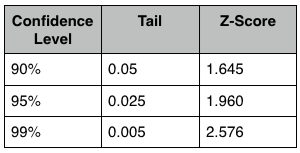
- Confidence levels and z- scores are retrieved from a given chart below:
 RSS Feed
